OpenCV+TensorFlow 人工智能图像处理 (1)

1. OpenCV初识

OpenCV是一个开源的计算机视觉库，OpenCV是一个基于BSD许可（开源）发行的跨平台计算机视觉库，可以运行在Linux、Windows、Android和Mac OS操作系统上。它轻量级而且高效——由一系列 C 函数和少量 C++ 类构成，同时提供了Python、Ruby、MATLAB等语言的接口，实现了图像处理和计算机视觉方面的很多通用算法。

主要应用场景：指纹识别，自动驾驶，人脸识别等。

2. Tensorflow 初识

TensorFlow是谷歌基于DistBelief进行研发的第二代人工智能学习系统，其命名来源于本身的运行原理。Tensor（张量）意味着N维数组，Flow（流）意味着基于数据流图的计算，TensorFlow为张量从流图的一端流动到另一端计算过程。TensorFlow是将复杂的数据结构传输至人工智能神经网中进行分析和处理过程的系统。

3. Hello World

import tensorflow as tf
# 先运行，之后就有代码提示了

hello = tf.constant('hello tensorflow!')
sess = tf.Session()
# 使用print时必须使用session
print(sess.run(hello))

b'hello tensorflow!'

import cv2
print('hello opencv!')

hello opencv!

4. 图片的读取和展示

# cv 读取图片， 先读取图片，在展示出来， 再暂停窗口
import cv2
img = cv2.imread('images/image0.jpg', 1) # 图片的读取，第二个参数表示读取图片的类型，0： gray图   1： color图
cv2.imshow('image', img) # 窗口的title， 需要展示的内容
cv2.waitKey(0)

1048603

5. OpenCV模块组织结构

官网：https://opencv.org/

• calib3d: 主要用于3D
• core： 非常重要记录了OpenCV的基础数据类型，矩阵操作，绘图相关
• dnn： 神经网络相关
• features2d： 图形焦点相关，如图像匹配的时候需要使用
• flann： 聚类相关
• highgui： 图形交互界面
• imgcodecs, imgproc： 非常重要 图形处理相关，如滤波器，直方图统计，均衡化，集合变换，颜色处理
• ml： 非常重要 机器学习模块
• objdetect： 物体检测
• photo： 非常重要 图片处理，如，图片修复，去噪
• shape： 形状
• stitching： 拼接模块，主要用于大图像拼接
• video, videoio, videostab： 视频信息，视频分解图像，图像合成视频等

6. 图像写入

import cv2
# 1. 文件的读取   2. 封装格式解析   3. 数据解码   4. 数据加载
img = cv2.imread('images/image0.jpg', 1)
# png jpg 这些都是文件的压缩格式，通过压缩格式使用对应的解码器可以解码图片
cv2.imshow("image", img)

cv2.waitKey(0)

-1

import cv2
img = cv2.imread("images/image0.jpg", 1)
cv2.imwrite('images/image1.jpg', img) # 第一个参数是图片的路径，需要加上图片的类型（拓展名）  第二个参数是写入的数据

True

7. 不同质量图片保存

import cv2
img = cv2.imread('images/image0.jpg', 1)
cv2.imwrite('images/imageTest.jpg', img, [cv2.IMWRITE_JPEG_QUALITY, 10]) # 第三个参数指定图像写入时的质量，质量范围是0-100 【有损压缩】

True

# 压缩成png   png相比jpg的特点： png 无损压缩， png可以设置图像的透明度
import cv2
img = cv2.imread('images/image0.jpg', 1)
cv2.imwrite('images/imageTest.png', img, [cv2.IMWRITE_PNG_COMPRESSION, 0]) # compression 压缩比[0-9]

True

8. 像素相关

像素：组成图片的元素，由1个RGB组成

RGB：组成颜色的元素，R: red, G: green, B: blue

颜色深度： 比如8bit的颜色深度： 可以表示0-255种颜色

图片的宽高： 表示图片在水平和垂直方向上有多少像素点

图片大小计算： 1.14M = 720*547*3*8 bit / 8 (B) = 1.14M 宽， 高， RGB3个值， 颜色深度， 这里bit要转成B，再从B转为M

PNG图片大小： PNG图片还有一个alpha通道，透明属性通道

BGR： OpenCV种经常这样表示， blue green red

9. 像素操作

import cv2
img = cv2.imread('images/image0.jpg', 1)
(b, g, r) = img[100, 100]  # BGR是一个元组格式
print(b, g, r)
# 在（10， 100） -> （110， 100）处绘制直线
# for i in range(100):
#     img[10+i, 100] = (255, 0, 0)
img[10:100, 100] = (255, 0, 0)
cv2.imshow("image", img)
cv2.waitKey(0) # 指定0，直到用户输入程序才会继续执行，如果指定1000， 程序会在1000ms=1s后继续执行

39 46 49





-1

10. Tensorflow的常量与变量

import tensorflow as tf
# 常量
# data1 = tf.constant(2.5)
data1 = tf.constant(2, dtype=tf.int32)
# 变量
data2 = tf.Variable(10, name='var') # 变量的内容设置为10， 变量name为var
print (data1)
print (data2)
'''
sess = tf.Session()
print(sess.run(data1))
# 变量需要初始化之后才能使用
init = tf.global_variables_initializer()
sess.run(init)
print(sess.run(data2))
sess.close()
'''
init = tf.global_variables_initializer()
with tf.Session() as sess:
    sess.run(init)
    print(sess.run(data2))

Tensor("Const_7:0", shape=(), dtype=int32)
<tf.Variable 'var_6:0' shape=() dtype=int32_ref>
10

11. Tensorflow的工作机制

Tensorflow的实质：张量Tensor + 计算图Graphs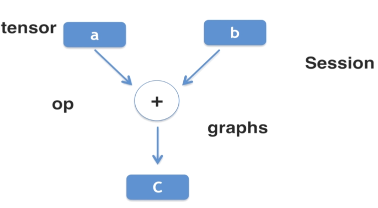

12. tf的四则运算

# 常量
import tensorflow as tf
data1 = tf.constant(6)
data2 = tf.constant(2)
dataAdd = tf.add(data1, data2)
dataSub = tf.subtract(data1, data2)
dataMul = tf.multiply(data1, data2)
dataDiv = tf.divide(data1, data2)

with tf.Session() as sess:
    print(sess.run(dataAdd))
    print(sess.run(dataSub))
    print(sess.run(dataMul))
    print(sess.run(dataDiv))

8
4
12
3.0

# 变量
import tensorflow as tf
data1 = tf.constant(6)
data2 = tf.Variable(2)
dataAdd = tf.add(data1, data2)
# 数据拷贝
dataCopy = tf.assign(data2, dataAdd) # 把dataAdd的结果赋予给data2
dataSub = tf.subtract(data1, data2)
dataMul = tf.multiply(data1, data2)
dataDiv = tf.divide(data1, data2)
init = tf.global_variables_initializer()

with tf.Session() as sess:
    sess.run(init)
    print(sess.run(dataAdd))
    print(sess.run(dataSub))
    print(sess.run(dataMul))
    print(sess.run(dataDiv))
    print('sess.run(dataCopy)', sess.run(dataCopy))
    print('dataCopy.eval()', dataCopy.eval())   # 执行运算图
    print('tf.get_default_session()', tf.get_default_session().run(dataCopy))

8
4
12
3.0
sess.run(dataCopy) 8
dataCopy.eval() 14
tf.get_default_session() 20

13. tf矩阵基础

# 使用placehold， 先定义变量，后赋值
import tensorflow as tf
data1 = tf.placeholder(tf.float32)
data2 = tf.placeholder(tf.float32)
dataAdd = tf.add(data1, data2)
with tf.Session() as sess:
    print(sess.run(dataAdd, feed_dict={data1:6, data2: 2.2}))
    # feed_dice: 字典类型，给placehold赋值

8.2

# 矩阵
import tensorflow as tf
# 1行2列
data1 = tf.constant([[6, 6]])
# 2行1列
data2 = tf.constant([[2], [2]])
data3 = tf.constant([[3, 3]])
# 3x2
data4 = tf.constant([[1, 2], 
                     [3, 4], 
                     [5, 6]])
print(data4.shape) # 打印矩阵的纬度

with tf.Session() as sess:
    print(sess.run(data4))
    print(sess.run(data4[0, 1]))  # 中括号第一个表示行，第二个表示列

(3, 2)
[[1 2]
 [3 4]
 [5 6]]
2

# 矩阵的运算
import tensorflow as tf
data1 = tf.constant([[6, 6]])
data2 = tf.constant([[2], 
                     [2]])
data3 = tf.constant([[3, 3]])
data4 = tf.constant([[1, 2], 
                     [3, 4], 
                     [5, 6]])
matMul = tf.matmul(data1, data2)
matMul2 = tf.multiply(data1, data2)
matAdd = tf.add(data1, data3)
with tf.Session() as sess:
#     print(sess.run(matMul))
#     print(sess.run(matAdd))
#     print(sess.run(matMul2))
    print(sess.run([matMul, matAdd, matMul2]))

[array([[24]]), array([[9, 9]]), array([[12, 12],
       [12, 12]])]

# 特殊矩阵
import tensorflow as tf
mat0 = tf.constant([[0, 0, 0], [0, 0, 0]])
mat1 = tf.zeros([2, 14])
mat2 = tf.ones([3, 2])
mat3 = tf.fill([3, 2], 15) # 使用某个值填充
with tf.Session() as sess:
#     print(sess.run(mat0))
#     print(sess.run(mat1))
#     print(sess.run(mat2))
    print(sess.run(mat3))

[[15 15]
 [15 15]
 [15 15]]

import tensorflow as tf
mat1 = tf.constant([[2], [3], [4]])
mat2 = tf.zeros_like(mat1)
mat3 = tf.linspace(0.0, 2.0, 11)
mat4 = tf.random_uniform([2, 3], -1, 2) # 产生2x3的随机矩阵，矩阵值范围：[-1 - 2)
with tf.Session() as sess:
#     print(sess.run(mat2))
#     print(sess.run(mat3))
      print(sess.run(mat4))

[[ 0.44656682 -0.9664166  -0.21917105]
 [-0.62286747 -0.39322567 -0.81225216]]

14. Numpy基础

import numpy as np
data1 = np.array([1, 2, 3, 4, 5])
print (data1)

[1 2 3 4 5]

data2 = np.array([[1, 2], [3, 4]])
print (data2)
print (data2.shape)

[[1 2]
 [3 4]]
(2, 2)

# zero ones
print (np.zeros([3, 2]))
print (np.ones([2, 2]))

[[0. 0.]
 [0. 0.]
 [0. 0.]]
[[1. 1.]
 [1. 1.]]

# 矩阵的修改与查找
data2[1, 0] = 6
print (data2)
print (data2[1, 1])

[[1 2]
 [6 4]]
4

# 基本运算
data3 = np.ones([2, 3])
print (data3 * 2) # 对应相乘
data4 = np.array([[1, 2, 3], [4, 5, 6]])
print (data3 + data4) # 矩阵对应相加
print (data3 * data4)
a = np.array([[1, 2], [2, 1]])
b = np.array([[1, 2], [2, 2]])
print (a * b)  # 对应元素相乘
print (a.dot(b)) # 矩阵的乘法

[[2. 2. 2.]
 [2. 2. 2.]]
[[2. 3. 4.]
 [5. 6. 7.]]
[[1. 2. 3.]
 [4. 5. 6.]]
[[1 2]
 [2 1]]
[[1 2]
 [2 1]]
[[1 4]
 [4 2]]
[[5 6]
 [4 6]]

15. Matplotlib基础

import numpy as np
import matplotlib.pyplot as plt

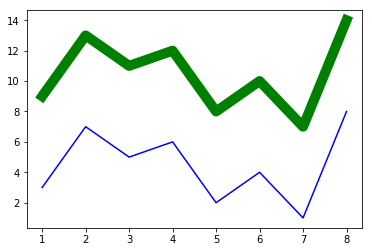
# 折线图
x = np.array([1, 2, 3, 4, 5, 6, 7, 8])
y = np.array([3, 7, 5, 6, 2, 4, 1, 8])
plt.plot(x, y, 'b') # 绘制折线图  x y 颜色
plt.plot(x, y+6, 'g', lw=10) # lw 线条的宽度(line width)

[<matplotlib.lines.Line2D at 0x7f660c1fccf8>]

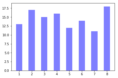
# 柱状图
x = np.array([1, 2, 3, 4, 5, 6, 7, 8])
y = np.array([13, 17, 15, 16, 12, 14, 11, 18])
plt.bar(x, y, 0.5, alpha=0.5, color='b') # 第三个参数：每个柱子的宽度，占一格的百分数  alpha:透明度，保存png图片的时候才有效

<BarContainer object of 8 artists>

# 饼图
labels = ['p1', 'p2', 'p3']
sizes = [60, 30, 10]
colors = ['red', 'green', 'blue']
plt.pie(sizes, labels=labels, colors=colors,
        labeldistance = 1.1,autopct = '%3.1f%%',shadow = False,
        startangle = 90,pctdistance = 0.6)
#labeldistance，文本的位置离远点有多远，1.1指1.1倍半径的位置
#autopct，圆里面的文本格式，%3.1f%%表示小数有三位，整数有一位的浮点数
#shadow，饼是否有阴影
#startangle，起始角度，0，表示从0开始逆时针转，为第一块。一般选择从90度开始比较好看
#pctdistance，百分比的text离圆心的距离
#patches, l_texts, p_texts，为了得到饼图的返回值，p_texts饼图内部文本的，l_texts饼图外label的文本

([<matplotlib.patches.Wedge at 0x7f66004ee240>,
  <matplotlib.patches.Wedge at 0x7f66004ee9b0>,
  <matplotlib.patches.Wedge at 0x7f6600476198>],
 [Text(-1.04616,-0.339919,'p1'),
  Text(1.1,2.05979e-07,'p2'),
  Text(0.339918,1.04616,'p3')],
 [Text(-0.570634,-0.18541,'60.0%'),
  Text(0.6,1.12352e-07,'30.0%'),
  Text(0.18541,0.570634,'10.0%')])

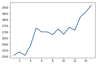
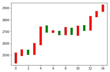
16. 实战：人工神经网络逼近股票收盘均价

import numpy as np
import tensorflow as tf
import matplotlib.pyplot as plt

# y轴表示日期
date = np.linspace(1, 15, 15)
# 收盘价
endPrice = np.array([2511.90,2538.26,2510.68,2591.66,2732.98,2701.69,2701.29,2678.67,2726.50,2681.50,2739.17,2715.07,2823.58,2864.90,2919.08])
# 开盘价
startPrice = np.array([2438.71,2500.88,2534.95,2512.52,2594.04,2743.26,2697.47,2695.24,2678.23,2722.13,2674.93,2744.13,2717.46,2832.73,2877.40])
# 绘图
plt.figure()
for i in range(15):
    # 柱状图
    dataOne = np.zeros([2])
    dataOne[0] = i
    dataOne[1] = i
    priceOne = np.zeros([2])
    priceOne[0] = startPrice[i]
    priceOne[1] = endPrice[i]
    if endPrice[i] > startPrice[i]:
        plt.plot(dataOne, priceOne, 'r', lw=8)
    else:
        plt.plot(dataOne, priceOne, 'g', lw=8)

# 搭建神经网络
# 输入日期，输出股价
# A(15*1) * w1(1*10) + b1(1*10) = B(15*10)
# B(15*10) * w2(10*1) + b2(15*1) = C(15*1)
# 为了计算方便，将日期进行归一化
dateNormal = np.zeros([15, 1])
priceNormal = np.zeros([15, 1])
for i in range(15):
    dateNormal[i] = i / 14.0
    priceNormal[i] = endPrice[i] / 3000.0

# 定义输入层
x = tf.placeholder(tf.float32, [None, 1]) # 表面n行1列
y = tf.placeholder(tf.float32, [None, 1])

# 定义隐藏层
w1 = tf.Variable(tf.random_uniform([1, 10], 0, 1)) # 创建w1， 初始数据在0~1范围内， 因为神经网络需要对其进行更新，所以是变量
b1 = tf.Variable(tf.zeros([1, 10]))
# 定义一个操作
wb1 = tf.matmul(x, w1) + b1
layer1 = tf.nn.relu(wb1) # 激励函数

# 定义输出层
w2 = tf.Variable(tf.random_uniform([10, 1], 0, 1))
b2 = tf.Variable(tf.zeros([15, 1]))
wb2 = tf.matmul(layer1, w2) + b2
layer2 = tf.nn.relu(wb2)

# 定义神经网络输出与实际值的差异，为了调整循环次数
loss = tf.reduce_mean(tf.square(y-layer2)) # y是真实值  这行代码实际是运算了标准差
train_step = tf.train.GradientDescentOptimizer(0.1).minimize(loss) # 梯度下降，步长，最小化loss

# 运行神经网络
with tf.Session() as sess:
    sess.run(tf.global_variables_initializer()) # 变量初始化
    for i in range(10000):
        sess.run(train_step, feed_dict={x:dateNormal, y:priceNormal})
    pred = sess.run(layer2, feed_dict={x:dateNormal})
    predPrice = np.zeros([15, 1])
    for i in range(15):
        predPrice[i] = pred[i]*3000

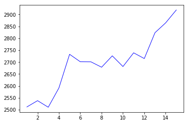
plt.plot(date, predPrice, 'b', lw=2)
plt.plot(date, endPrice, 'g', lw=1)

[<matplotlib.lines.Line2D at 0x7fef4481f908>]